Criterion B Details

# Default ecosystem code for template development.
# This line is replaced by build_ecosystem_pages.py for each ecosystem.
ecosystem_code = 'Coralino Oceanico'

Import Python modules.

import os
import yaml
from pathlib import Path
from lonboard import Map
from rle.core import Ecosystems, criterion_b_status, rle_category
from rle.core.eoo import make_eoo
from rle.core.aoo import make_aoo_grid

Load the country config file.

project_root = os.environ.get('PIXI_PROJECT_ROOT', str(Path('..').resolve()))
config_path = Path(project_root) / 'config' / 'country_config.yaml'
with open(config_path) as f:
    config = yaml.safe_load(f)

# Ecosystem index (the COG pixel value for this ecosystem), looked up by code
# from the canonical index table. Absent if the index has not been built yet.
import csv
ecosystem_index = None
index_csv = Path(project_root) / 'config' / 'ecosystems' / 'index.csv'
if index_csv.exists():
    with open(index_csv) as f:
        for row in csv.DictReader(f):
            if row['code'] == ecosystem_code:
                ecosystem_index = int(row['index'])
                break

Load & Filter Ecosystem Data

Load data for all the ecosystems.

import sys
# Shared config helpers live in scripts/; make them importable from here.
sys.path.insert(0, str(Path(project_root) / 'scripts'))
from _config import ensure_vector_source

source = config['ecosystem_source']
# ecosystem_code_column is optional: fall back to the name column.
ecosystem_column = source.get('ecosystem_code_column') or source.get('ecosystem_name_column')
# Prefer the ecosystem-sorted `optimized_data` copy when configured, so that
# filtering to one ecosystem uses parquet predicate pushdown instead of loading
# the whole national map into memory. Falls back to `data`.
ecosystems = Ecosystems.from_file(
    ensure_vector_source(source.get('optimized_data') or source['data']),
    ecosystem_column=ecosystem_column,
    ecosystem_name_column=source.get('ecosystem_name_column'),
    functional_group_column=source.get('functional_group_column')
)

Filter by the Coralino Oceanico and check the number of features.

ecosystem = ecosystems.filter(ecosystem_code)
has_data = ecosystem.size() > 0
print(f'{ecosystem.size() = }')
if not has_data:
    from IPython.display import Markdown, display
    display(Markdown(
        f'**No spatial data found for {ecosystem_code}.** '
        f'Criterion B calculations are skipped.'
    ))

ecosystem.size() = 1277

Extent of Occurrence (EOO) (subcriterion B1)

Extent of occurrence (EOO). The EOO of an ecosystem is the area (km2) of a minimum convex polygon – the smallest polygon in which no internal angle exceeds 180° that encompasses all known current spatial occurrences of the ecosystem type.

The minimum convex polygon (also known as a convex hull) must not exclude any areas, discontinuities or disjunctions, regardless of whether the ecosystem can occur in those areas or not. Regions such as oceans (for terrestrial ecosystems), land (for coastal or marine ecosystems), or areas outside the study area (such as in a different country) must remain included within the minimum convex polygon to ensure that this standardised method is comparable across ecosystem types. In addition, these features contribute to spreading risks across the distribution of the ecosystem by making different parts of its distribution more spatially independent.

Calculate EOO

Start by calculating the convex hull of the ecosystem’s distribution.

import geopandas as gpd

if has_data:
    ecosystem_geometry = ecosystem.geometry.union_all()
    gdf_ecosystem_polygons = gpd.GeoDataFrame(geometry=[ecosystem_geometry], crs=ecosystem.geometry.crs)
    hull = ecosystem_geometry.convex_hull
    gdf_hull = gpd.GeoDataFrame(geometry=[hull], crs=ecosystem.geometry.crs)

Display the ecosystem’s distribution and the convex hull.

from lonboard import Map, PolygonLayer
from rle.core.viz import smart_map

if has_data:
    eoo_hull = make_eoo(ecosystem).compute()
    display(smart_map([eoo_hull, ecosystem]))

/home/runner/work/rle-tyler-colombia/rle-tyler-colombia/.pixi/envs/default/lib/python3.11/site-packages/lonboard/_geoarrow/ops/reproject.py:116: UserWarning: Input being reprojected to EPSG:4326 CRS.
Lonboard is only able to render data in EPSG:4326 projection.
  warnings.warn(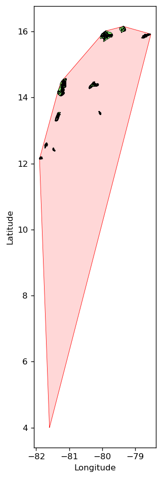

if has_data:
    hull_ea = gdf_hull.to_crs("ESRI:54034")
    eoo = hull_ea.geometry.iloc[0].area / 1e6
    print(f'EOO is {eoo:.1f} km2')

EOO is 222112.9 km2

Then calculate the area of the convex hull polygon.

Direct calculation of EOO

EOO can also be calculated directly using …

if has_data:
    ecosystem.eoo

Verify that the area returned by calling make_eoo(ecosystem).compute().area_km2 is the same as the area of the convex hull polygon.

if has_data:
    assert ecosystem.eoo == eoo

Area of Occupancy (AOO) (subcriterion B2)

The protocol for this adjustment includes the following steps:

Intersect AOO grid with the ecosystem’s distribution map.

Calculate extent of the ecosystem type in each grid cell (area) and sum these areas to obtain the total ecosystem area (total area).

Arrange grid cells in ascending order based on their area (smaller first). Calculate accumulated sum of area per cell (cumulative area).

Calculate cumulative proportion by dividing cumulative area by total area (cumulative proportion takes values between 0 and 1)

Calculate AOO by counting the number of cells with a cumulative proportion greater than 0.01 (i.e. exclude cells that in combination account for up to 1% of the total mapped extent of the ecosystem type).

AOO Calculation Details

Intersect AOO grid and ecosystem map

Intersect AOO grid with the ecosystem’s distribution map

from pathlib import Path
from rle.core.aoo import make_aoo_grid_cached

if has_data:
    # Prefer a prebuilt grid cache (e.g. a gs:// URI) so the national AOO grid
    # is not recomputed during CI renders — computing it from the full national
    # ecosystem map peaks at many GB of RAM. Fall back to a local cache when no
    # prebuilt cache is configured. Build one with `pixi run build-caches`.
    cache_path = (
        source.get('aoo_grid_cache_url')
        or (Path(project_root) / '.cache' / 'aoo_grid.parquet')
    )
    aoo_grid = make_aoo_grid_cached(ecosystems, cache_path=cache_path)
    aoo_grid_filtered = aoo_grid.filter_by_ecosystem(ecosystem_code)

Visualize variations in the AOO grid.

from matplotlib.colors import LinearSegmentedColormap
from lonboard.colormap import apply_continuous_cmap
from rle.core.aoo import slugify_ecosystem_name

ecosystem_column = slugify_ecosystem_name(ecosystem_code)
if has_data:
    cmap = LinearSegmentedColormap.from_list("white_red", ["white", "red"])
    values = aoo_grid_filtered.grid_cells[ecosystem_column].values
    normalized = (values - values.min()) / (values.max() - values.min())
    colors = apply_continuous_cmap(normalized, cmap)
    display(smart_map([(aoo_grid_filtered, {"get_fill_color": colors}), ecosystem]))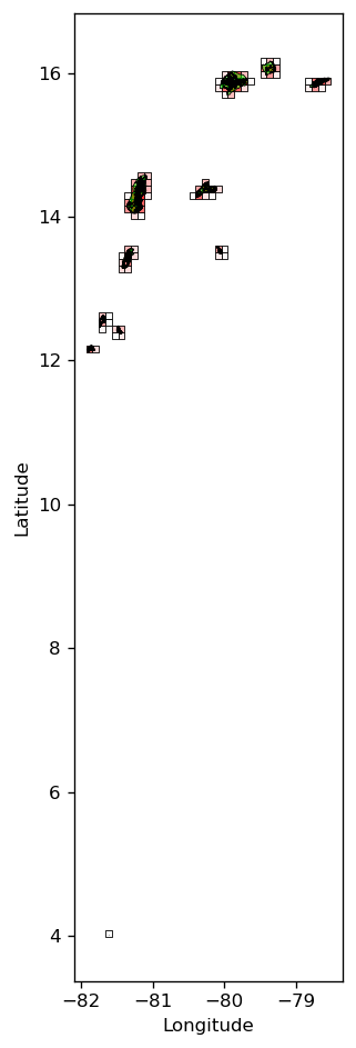

Calculate grid cell area and total area

Calculate extent of the ecosystem type in each grid cell (area) and sum these areas to obtain the total ecosystem area (total area).

if has_data:
    keep = ['geometry', 'grid_col', 'grid_row', ecosystem_column]
    gdf = aoo_grid_filtered.grid_cells[keep]
    display(gdf)

	geometry	grid_col	grid_row	Coralino_Oceanico
0	POLYGON ((-81.83652 12.11584, -81.83652 12.208...	-912	133	0.494131
1	POLYGON ((-81.74669 12.11584, -81.74669 12.208...	-911	133	0.143380
2	POLYGON ((-81.65686 12.39331, -81.65686 12.485...	-910	136	0.032338
3	POLYGON ((-81.65686 12.48587, -81.65686 12.578...	-910	137	0.368507
4	POLYGON ((-81.65686 12.57845, -81.65686 12.671...	-910	138	0.243988
...	...	...	...	...
82	POLYGON ((-78.69242 15.74756, -78.69242 15.841...	-877	172	0.408114
83	POLYGON ((-78.69242 15.84145, -78.69242 15.935...	-877	173	0.519981
84	POLYGON ((-78.60259 15.74756, -78.60259 15.841...	-876	172	0.069754
85	POLYGON ((-78.60259 15.84145, -78.60259 15.935...	-876	173	0.653503
86	POLYGON ((-78.51276 15.84145, -78.51276 15.935...	-875	173	0.337137

87 rows × 4 columns

The column Coralino_Oceanico contains the (fractional) area of the ecosystem in each grid cell.

Sum up the areas of each grid cell to get the total area.

if has_data:
    total_area = gdf[ecosystem_column].sum()
    display(total_area)

np.float64(31.373430005281314)

Calculate cumulative area

Arrange grid cells in ascending order based on their area (smaller first). Calculate accumulated sum of area per cell (cumulative area).

if has_data:
    gdf = gdf.sort_values(by=ecosystem_column)
    gdf["cumulative_area"] = gdf[ecosystem_column].cumsum()
    display(gdf)

	geometry	grid_col	grid_row	Coralino_Oceanico	cumulative_area
5	POLYGON ((-81.56703 3.98235, -81.56703 4.073, ...	-909	44	0.000063	0.000063
7	POLYGON ((-81.56703 12.57845, -81.56703 12.671...	-909	138	0.000250	0.000313
81	POLYGON ((-78.78225 15.84145, -78.78225 15.935...	-878	173	0.000347	0.000660
41	POLYGON ((-80.39922 14.25083, -80.39922 14.344...	-896	156	0.000532	0.001192
30	POLYGON ((-81.11787 13.9713, -81.11787 14.0644...	-904	153	0.001301	0.002493
...	...	...	...	...	...
62	POLYGON ((-79.86023 15.84145, -79.86023 15.935...	-890	173	1.000000	27.373430
65	POLYGON ((-79.7704 15.84145, -79.7704 15.93538...	-889	173	1.000000	28.373430
26	POLYGON ((-81.2077 14.15761, -81.2077 14.25083...	-905	155	1.000000	29.373430
34	POLYGON ((-81.11787 14.34408, -81.11787 14.437...	-904	157	1.000000	30.373430
75	POLYGON ((-79.32124 16.02936, -79.32124 16.123...	-884	175	1.000000	31.373430

87 rows × 5 columns

Calculate cumulative proportion

Calculate cumulative proportion by dividing cumulative area by total area (cumulative proportion takes values between 0 and 1)

if has_data:
    gdf["cumulative_proportion"] = gdf["cumulative_area"] / total_area
    display(gdf)

	geometry	grid_col	grid_row	Coralino_Oceanico	cumulative_area	cumulative_proportion
5	POLYGON ((-81.56703 3.98235, -81.56703 4.073, ...	-909	44	0.000063	0.000063	0.000002
7	POLYGON ((-81.56703 12.57845, -81.56703 12.671...	-909	138	0.000250	0.000313	0.000010
81	POLYGON ((-78.78225 15.84145, -78.78225 15.935...	-878	173	0.000347	0.000660	0.000021
41	POLYGON ((-80.39922 14.25083, -80.39922 14.344...	-896	156	0.000532	0.001192	0.000038
30	POLYGON ((-81.11787 13.9713, -81.11787 14.0644...	-904	153	0.001301	0.002493	0.000079
...	...	...	...	...	...	...
62	POLYGON ((-79.86023 15.84145, -79.86023 15.935...	-890	173	1.000000	27.373430	0.872504
65	POLYGON ((-79.7704 15.84145, -79.7704 15.93538...	-889	173	1.000000	28.373430	0.904378
26	POLYGON ((-81.2077 14.15761, -81.2077 14.25083...	-905	155	1.000000	29.373430	0.936252
34	POLYGON ((-81.11787 14.34408, -81.11787 14.437...	-904	157	1.000000	30.373430	0.968126
75	POLYGON ((-79.32124 16.02936, -79.32124 16.123...	-884	175	1.000000	31.373430	1.000000

87 rows × 6 columns

Count AOO cells

Calculate AOO by counting the number of cells with a cumulative proportion greater than 0.01 (i.e. exclude cells that in combination account for up to 1% of the total mapped extent of the ecosystem type).

if has_data:
    aoo = len(gdf[gdf["cumulative_proportion"] > 0.01])
    print(f'AOO is {aoo} cells')

AOO is 69 cells

AOO Calculation (direct call)

if has_data:
    aoo_count = ecosystem.aoo
    print(f'AOO: {aoo_count} grid cells')

AOO: 69 grid cells

Criterion B Summary

Criterion B status (spatial)

Least Concern (LC) — Coralino Oceanico (Coralino Oceanico), index 42

Status reflects the spatial thresholds for EOO (B1) and AOO (B2) only. A final listing under B1/B2 additionally requires at least one of: (a) an observed or inferred continuing decline; (b) threatening processes likely to cause continuing decline within 20 years; or (c) few threat-defined locations — none of which are derived from the spatial metrics.

Sub-criterion	Metric	Value	Category
B1	EOO	222113 km²	Least Concern (LC)
B2	AOO	69 cells	Least Concern (LC)
Overall B	—	—	Least Concern (LC)